Artificial Intelligence

Definition: The study and design of intelligent agents, where an intelligent agent is a system that perceives its environment and takes actions that maximize its chances of success.

---

Agent and environment:

Rational agent: The agent which selects the action that maximizes its performance measure given its inputs or perceptions and built-in knowledge.

PEAS: Performance, Environment, Actuators, and Sensors

Types of Environment:

1. Fully vs partially observable:
2. Deterministic( vs stochastic): The next state of the environment is completely determined by the current state.
3. Episodic vs sequential: Each perception-action pair can be considered as an episode.
4. static vs dynamic:
5. discrete vs continuous:
6. single-agent vs multi-agent:
7. known vs unknown:

Types of Agents in the order of increasing generality:

1. Simple reflex agents: based on current state only. Look up the table of percepts and actions.
2. Model-based reflex agents: based on percept history, maintains a model of the world, condition-action rules decide the action of the agent.
3. Goal-based agents: contains goal information additional to Model-based agents.Goals decide the actions of the agent.
4. Utility-based agents:  Utility function is the agent’s performance measure. try to increase the happiness.
5. Learning agents:

Agent’s organisation:

1. Atomic representation: Consider each state as a black box.
2. Factored representation: Each state has attribute value properties.
3. Structured representation: Relationship between objects inside a state.

Search Agents

General example problems from AI textbook:

1. Travelling salesman problem.
2. Route finding problem
3. Robot navigation
4. protein design

State space, search space and search tree.

Measures:

1. Completeness: Can the algorithm find a solution when there exists one?
2. Optimality: Can the algorithm find the least cost path to the solution?
3. Time complexity: How long does it take to complete the search.
4. Space complexity: How much memory is needed to complete the search.

Two types of search:

1. Uninformed: No information about the domain.
   1. Breadth-first: FIFO
      1. 
      2. Applications: computing shortest path when all the edge lengths are same.
   2. Depth first: LIFO
      1. 
      2. Depth limited is not optimal because it might return us a high-cost path on the left sub-tree without considering other low-cost paths in the right subtree.
      3. Applications: Topological ordering of directed acyclic graphs.
   3. Depth limited: Depth first with depth limit
   4. Iterative deepening: Depth limited with increasing limit, combines benefits of depth first and breadth first. First do depth first search to a depth limit n and then increase the depth and do depth first search again. diff of BFS and IDS
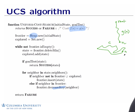
   5. Uniform cost: Expand least cost node first, FIFO
      1. Dijkstra’s algorithm is a variant of ucs, except that ucs finds shortest path from start node to goal node, whereas Dijkstra finds shortest path from start node to every other node.ucs and Djikshtra.Computing shortest path when edge lengths are different. Use heap data structure for speed.
      2. I doubt Google uses UCS for it’s route finding in maps. Cost between the nodes can be a mix of distance, traffic, weather etc.Maps algorithm
         1. 
2. Informed: Some information about the domain and goals.
   1. Heuristics search (h(n)): Determine how close we are to the goal based on a heuristic function. Admissible heuristic thinks that the cost to the solution is less than the actual cost.
      1. Greedy search expands the node that appears to be closest to the goal. uses a heuristic function that has the information of cost from a particular node to the target node.
         1. 
      2. A* search:  Consider both the heuristic that says about the cost from a node to the target node and cost to reach that node. A* search will revise it’s decision, whereas greedy search would not. This property makes greedy incomplete and A* complete.
      3. IDA*:
3. Local search: iterative improvement algorithms by an optimization/fitness function.
   1. Hill climbing (steepest descent/ascent,greedy local search):some variants of this are:
      1. sideways moves – escape flat lines.
      2. Random restart – to overcome local maxima.
      3. Stochastic –
   2. Simulated annealing : from statistical physics.
   3. Local beam search – k states instead of single state.
   4. Genetic algorithms: from evolutionary biology
      1. 

Adversarial search and games:

Multiagent environment, uncontrollable opponent.

Not a sequence of actions, but a strategy or policy.

Approximation is the key ingredient in the face of combinatorial explosion.

(perfect information, deterministic) – Zero sum games.

At any stage, one agent will try to pick the move with maximum utility out of all legal moves and the opponent will pick the move with minimum utility.

Embedded thinking or backward reasoning:

Thinking through the consequences and potential actions of the opponent before making the decision.

Minimax : Two opponents playing optimally, one trying to maximize and other trying to minimize the utility.

Alpha-Beta pruning:

When the agent that is trying to find Max utility of it’s children, you start with an alpha as (-infinity), and update alpha if you find any child nodes with utility better than present alpha. During this process, if you come across any 2nd gen childs with utility less than alpha, then you don’t need look for utilities of other 2nd gen childs of that particular 1st child. Why? because that 1st gen child is trying to find minimum, once you go down below alpha, that 1st gen child is out context at the zeroth generation which is trying to find max has found that this 1st gen child can no longer contribute to me. In this context, ordering of child nodes matters a lot. Right ordering can save you from exploring a lot of unnecessary childs/paths.

Stochastic/Non-deterministic games:

A chance/random element involved.

Expectiminimax.

Machine Learning:

Data collection -> Data preparation -> Exploratory Data analysis(picture the data using different graphs and charts) -> Machine learning techniques -> Visualization -> Decision

1. Decision trees:
2. Rule induction:
3. Neural networks:
4. SVMs
5. Clustering method
   1. K-means
   2. Gaussian mixtures
   3. Hierarchical clustering
   4. Spectral clustering.
6. Association rules
7. Feature selection
8. Visualization
9. Graphical models
10. Genetic algorithm

Statistics:

1. Hypothesis testing
2. Experimental design
3. Anova
4. Linear regression
5. Logistic regression:
   1. It is a linear classifier, why?
      1. Because the decision boundary where the probability=0.5 is linear.
6. GLM
7. PCA

Definition of Machine learning:

A computer program is said to learn from experience E with respect to some class of tasks T and performance P, if its performance at tasks in T, as measured by P, improves with experience E.

BY its very definition, Machine learning algorithms are generally subdued to a particular class of tasks and not generic enough for general intelligence.

K-nearest neighbors:

O(n*d) – n is the number of training examples and d is the number of features.

K is usually chosen as odd value.

z-scaling – Each feature has a mean of 0 and a standard deviation of 1.

kernel regression is a flavor of k-nearest neighbors where we weight the contribution of each neighbor, whereas in k-nearest neighbor we just take the average.

Applications:

Recommender systems (collaborative filtering).

Breast cancer diagnosis

Handwritten character classification

information retrieval

---

 

To Avoid over fitting:

Reduce the number of features manually or do feature selection (Algorithms like random forest and XGBoost can give feature importance that you can use to prune less important features).

Do a model selection

Use regularization (keep the features but reduce their importance by setting small parameter values)

1. Lasso regularization (L1): used in case if you want to prune some unimportant features.
   1. 
2. Ridge regularization (L2): works better than L1 usually in practice.
   1. .

Do a cross-validation to estimate the test error.

Training set used for learning the model.

The validation set is used to tune the parameters, usually to control overfitting.

Linear Models:

1. Linear regression.
   1. Using least square loss
2. Linear classification:
   1. Perceptron: Data has to be linearly separable.

Classification: Logistic regression

Decision Trees: Tree classifiers

Start with a set of all our examples at the top root node.

Create branches considering splitting criteria and repeat this for creating other branches as you go down.

write the final decision at the bottom of the tree based on training examples and used this tree to classify any new test data.

First, we calculate entropy at a node and then compare info gains for extending that node for different dimensions. Then we choose to extend based on the category of high info gain.

Pruning strategies to escape overfitting:

1. Stop growing the tree earlier.
2. Grow a complex tree and then prune it back. Remove a subtree and check it against a validation set, if the performance doesn’t degrade, remove the subtree from the original.

Cart method:

Another method to build a decision tree.

1. Adopt same greedy, top-down algorithm.
2. Binary splits instead of multiway splits.
3. uses Gini index instead of information entropy.

Gini=1-p^2-P^2

p-proportion of positive examples

P-proportion of negative examples.

Bayes Rule:

Discriminative Algorithms:

Idea: Model p(y/x), conditional distribution of y given x.

Find a decision boundary that separates positive from negative example.

Generative Algorithms:

Naive Bayes assumes that feature values are conditionally independent given the label.

Naive Bayes classifier is linear.

Ensemble Methods:

An Ensemble method combines the predictions of many individual classifiers by majority voting.

Such individual classifiers, called weak learners, are required to perform slightly better than random.

1. Majority voting:
   1. Condorcet’s Jury theorem:
      1. Assumptions:
         1. Each individual makes the right choice with a probability p.
         2. The votes are independent.
      2. If p>0.5, then adding more voters increases the probability that the majority decision is correct. If p<0.5, then adding more voters makes things worse.
2. Boosting:
   1.  
   2. One of the most popular Machine learning methods.
   3. AdaBoost.M1-popular algorithm.
   4. Weak learners can be trees, perceptrons, decision stumps etc.
   5. The predictions of all weak learners are combined with a weighted majority voting.
   6. Idea: Train the weak learners on weighted training examples.
      1. AdaBoost with Decision stumps lead to a form of feature selection.
      2. Bootstrapping is a resampling technique for training weak learners from m samples of original training data.
   7. Iteratively give more weight on examples that are misclassified and less weight for examples that are classified properly.(Refer weight updation step d in above picture).
   8. 
   9. Boosting tends to avoid overfitting because of increasing margin as you add more and more weak learners.
   10. Boosting tends to overfit if weak learners themselves are overfitting.
3. Bagging:
   1. Bagging on trees works better than building a big tree on whole data.
4. Random forests: Make a lot of decision trees with each tree trained on a random subset of training data and a random subset of all features considered. use the majority votes of different decision trees to determine the final outcome for a random forest. This is relying on the principle that majority of decision trees will compensate for some wrongly classifying decision trees at different instances.
   1. Quora uses random forests for determining whether two questions are duplicates.

A practical guide to applying Support Vector Classification:

Clustering examples:

1. Clustering of the population by their demographics.
2. Audio signal separation.
3. Image segmentation.
4. Clustering of geographic objects
5. Clustering of stars.

Desirable clustering properties:

1. Richness: For any assignment of objects to clusters, there is some distance matrix D such that a clustering scheme returns that clustering. For example, Stop when clusters are x units apart reached is rich because it can address all possible clusterings with variations of x. On the other hand, stop when a fixed number of clusters reached, is not rich because it can’t address all possible clusters.
2. Scale invariance: Scaling distances by any value shouldn’t change the clustering of the objects.
3. Consistency: Shrinking(making similar things more similar) intra cluster distances and expanding(making non-similar things more non-similar) inter clustering distances shouldn’t change the clustering.

Impossibility theorem: No clustering algorithm can achieve all three of richness, scale invariance, and consistency.

K-means:

1. Based on initial conditions of the centroid, you may end up with totally different clusters. To deal with this, we take the ensemble of clusterings with different initializations. n_init parameter determines that.
2. sklearn.cluster.KMeans(n_clusters=8,max_iter=300, n_init=10).

Limitations of k-means:

1. Output for any given training set would always be same as long as we do not randomly pick initial centroids. But we usually choose centroids randomly in the beginning.
2. Hill climbing algorithm.

K-means fails for:

 

Solution for How to select K.

G-means:

How to evaluate?

internal evaluation: High intra-cluster similarity, Low inter-cluster similarity.

External evaluation: Mutual information, entropy, adjusted random index.

Other clustering methods:

1. Special clustering
2. DBSCAN
3. BIRCH

1.Single linkage clustering:

Keep on finding two closest points among all points and join them as long as you end up with k required clusters. This is a hierarchical agglomerative cluster structure.

Association Rules:

Supp(A->C): P(A^C)

Probabilistic interpretation:

R: A->C

conf(A->C)=P(C/A)=P(A^C)/P(A)

Though this looks like a valid measure, it doesn’t take into account P(C).

Interest(A->C)=P(A^C)/(P(A)*P(C))=Conf(A->C)/supp(C)

interest(R)=1 then A and C are independent.

interest(R)>1 then A and C are positively dependent.

interest(R)

Applications:

Collaborative filtering, customer behavior analysis, web organization, affinity promotion, cross-selling

Multidimensional rules:

Read more about Quantitative Association rules as well.

CONSTRAINT SATISFACTION PROBLEMS:

Care about goal rather than the path.

Three elements:

1. A set of variables.
2. A set of domains for each variable.
3. A set of constraints that specify allowable combinations of values.

Types of consistency:

1. Node consistency – unary constraints
2. Arc-consistency (Constraint propagation)- binary constraints – For every value that can be assigned to X, if there exists a value that can be assigned to Y, then X->Y is arc consistent. AC-3 is the algorithm that makes a CSP arc consistent. O(n^2*d^3)
3. Path-consistency – n-ary constraints

Forward checking propagates the information from assigned to unassigned variables only and does not check the interaction between unassigned variables. Arc consistency checks for all arcs and keep doing it whenever the domain of a variable is reduced. In this sense, AC is more general and an improvement of FC.

Two types of CSPs:

1. Search based
   1. BFS
   2. DFS
   3. BTS
2. Inference

Choose the one with minimum remaining values to fill first.

Fill with least constraining value first – the one that rules out fewest values in remaining variables.

Can work on independent subproblems separately based on the problem structure.

Backtracking:

d-size of domain, n-number of variables.

O(d^n)

Reinforcement learning:

Learning behaviour or actions based on the rewards/feedback from environment.

Science of sequential decision making.

1. Markov decision process – Formal model for sequential decision making.
   1. Markov property – Future is independent of the past given the current state.
   2. Applying reinforcement framework to Markov process.
   3. Theorem – Due to the Markov property, A discounted MDP always has the stationary optimal policy (pi).
   4. A policy is better than another policy if it’s value is greater than the other one calculated from all starting states.
   5. One useful fact is there always exist an optimal policy which is better than all other policies.
   6. Bellman equations.
   7. No closed form solution to Bellman equations to solve for optimal policy.
   8. other iterative solution approaches are
      1. Policy iteration.
      2. Value iteration.
   9. Think of different policies to traverse through MDP. Calculate value of each policy.
   10. Q-value iteration.
   11. Epsilon greedy exploration – with probability epsilon, take random action, with probability (1-epsilon) , take greedy action.

---

Logical agents or knowledge-based agents:

Mainly based on knowledge representation(domain specific) and inference(domain independent).

1. Using propositional logic.
2. Using First – Order Logic – used in personalized assistants.

pros and cons of Logical agents:

1. Doesn’t handle uncertainty, probability does.
2. Rule-based doesn’t use data, ML does.
3. It is hard to model every aspect of the world.
4. Models are encoded explicitly.

Resolution algorithm

Natural Language Processing:

Text classification (spam filtering)- Naive Bayes classifier.

Sentiment analysis

Naive bayes classifier – Assumes features are independent.

Classifies the new example based on the probabilities of different classes given the features of that particular example.

m-estimate of the probability:

1. Augment the sample size by m virtual examples, distributed according to prior p.

Chain rule of probability:

1. To estimate joint probability

N-gram model: Look N-1 words in the past to predict next word.

Bigrams capture synctactic dependencies such as noun comes after eat and verb comes after to etc.

3-grams and 4-grams are common in practice.

Perplexity – Hiigher the conditional probability, lower the perplexity.

Great progress:

Tagged text – which word is what type – noun, adjective,verb

Name entity recognition – yesterday(time), I(person), five (quantity)

Good progress:

Parsing – Exhibit the grammatical structure of a sentence.

Sentiment analysis – Does it identify sarcasm?

Machine translation

Information extraction.

work in progress:

Text summarization

Question/Answering

Dialog systems: Siri, echo etc.

---

Deep learning :

1. Less or no feature engineering required.
2. Need to choose number of layers in the stack and number of nodes in each layer.
3. Needs to be sensitive to minute details to distinguish between two breeds of a dog and at the same time, it should be invariant to large irrevelant variations like background, lighting and pose etc.
4. ReLU usually learns much faster in networks with many layers compared to sigmoid.
5. Pre-training was only needed for small data sets with the revival of deep learning.
6. Convnet combined with recurrent net to generate image captions. Vision to language interface.
7. Handwritten characters, spoken words, faces were most succesfull applications.
8. Theorem: No more than 2 hidden layers can represent any arbitrary region (assuming sufficient number of neurons or units).
9. The number of neurons in each hidden layer are found by cross validation.
10. The Mammalian visual cortex is hierarchical with 5-10 levels just for the visual system.
11. Examples of Deep neural networks – Restricted Boltzmann machines, convolutional NN, autoencoders etc.
12. Software for Deep learning:
    1. Tensorflow – Python
    2. Theano – Python
    3. Torch – LUA
    4. Caffe – Suited for vision

---

Robotics:

Path planning:

1. Visibility graph: VGRAPH – A-star search through the nodes between obstacles. guaranteed to give shortest path in 2d. Doesn’t scale well to 3d. Path close to obstacles (nodes at vertices).
2. Voronoi path planning:
3. Potential field path planning: Consider both robot and obstacles as positive charges repelling each other and Goal as negative charge attracting the robot. Take a Random walk in case you reach a local minimum.
4. Probabilistic roadmap planner: First needs to sample the space entirely and detect some collision free nodes. connect k nearest neighbor nodes. then do graph search to go from start to goal with these connected nodes. Can’t be sure that all nodes will be connected.

Glossary:

• Discriminative models learn the (hard or soft) boundary between classes
• Generative models model the distribution of individual class.
• Confusion matrix.
• ply – each move by one of the players.
• policy – State to action mapping
• stationary policy -Particular action for a particular state all the time.
• Representation learning – automatically discovers representations required to classify or predict, Not much feature engineering required. Ex: Deep learning.
• Saddle points/ minimax point – where derivative of the function is zero, but because of max in one ax and min in other axes. In the shape of the saddle on the horse.
• Unsupervised pre-training – Making features before feeding into the learning network.
• Configuration space(C – space): Set of parameters that completely describe the robot’s state. Proprioception.

CREDITS: Columbia University